Planning Inventory Purchases With Limited Capital: How to Split a Short Budget

Most inventory textbooks are written for a world where money isn’t the constraint. You calculate your reorder point, you calculate your optimal order quantity, and you buy. Simple. The problem is that almost no Mexican seller lives in that world. The month’s purchasing budget is a closed figure, it comes out of the cash on hand, and it always covers less than the spreadsheet suggests.

When the budget doesn’t cover everything, forecasting stops being an exercise in prediction and becomes an exercise in allocation. Knowing how much you’ll sell of each SKU is no longer enough: you have to decide which of all the SKUs that need replenishment get the money, and which go without this round. That second decision defines your year, and almost nobody makes it with a method.

What gets done instead, nearly always, is buying whatever ran out. You check inventory, you see what’s red, you order that. It’s intuitive and it’s an expensive mistake, because “what ran out” is a contaminated signal: things run out because they sell a lot, but also because you bought too little, because the lead time is long, because one big customer took them all at once. None of those three says anything about whether the item deserves your scarce capital.

This article proposes an explicit method. It isn’t sophisticated and it doesn’t require planning software: it requires three numbers per SKU and the discipline to rank them. The hard part isn’t the arithmetic, it’s accepting that some products won’t be restocked this cycle.

why “buy whatever ran out” splits the money badly

It’s worth taking the habit apart before replacing it, because it has an apparent logic that deceives.

Buying what’s out of stock optimizes exactly one thing: not having holes in the catalog. That’s a reasonable goal if your problem is visibility, because a listing without stock loses ranking and takes time to recover it. But when capital is the constraint, optimizing for “no holes” leads you to split the money evenly across products that don’t contribute equally.

The classic case: you have $400,000 to spend and 60 SKUs asking for replenishment. If you buy a little of each so none go empty, you end up with 60 products holding two weeks of coverage, all about to run out again, and next month you replay the same scene. That pattern — buying small and often so it stretches — raises your unit cost, costs you volume discounts, multiplies freight and leaves you permanently on the edge of a stockout across the whole catalog.

The uncomfortable but correct alternative is to concentrate. Buy properly into the products that justify it and accept that others come up short or get skipped. Concentrating hurts because it feels like abandoning products, and it is exactly what has to happen when money is finite.

the three inputs that order the decision

To decide which SKU gets the money, you need three things about each one. No more.

Sales velocity. How many units you move per day, measured over a window that represents current demand rather than an old spike. It’s what turns a quantity of units into a time horizon: 300 pieces of a product selling 10 a day is 30 days of inventory; the same 300 pieces of one selling 1 a day is ten months of sleeping capital.

Contribution per unit. What each unit leaves after subtracting everything the sale caused: channel commission, fulfillment, shipping, attributable advertising and a returns provision, on the pre-VAT base. Not gross margin. Gross margin lies in marketplaces because it ignores that the channel keeps a large slice of the sale.

Real lead time. How long the goods actually take from the moment you place the order to the moment they’re sellable on the channel. Not what the supplier promises: what you’ve measured, including customs, receiving, inbound to FBA or Full and the days the marketplace takes to make it available. Lead time doesn’t change whether a product deserves the money, but it does change when it needs it and how much has to be covered.

Glossary: sales velocity, units per day →

the metric that ranks: contribution per peso invested, per month

Those three inputs build the number worth ranking by. The idea is simple: scarce capital should go where it produces the most contribution per peso and per unit of time.

A product isn’t judged by what each sale leaves, but by what each peso invested in it leaves, and how many times a year that peso comes back around. A product with 40% contribution that turns twice a year yields less than one with 15% that turns eight times.

The math, per SKU:

1. Contribution per unit ÷ cost per unit. That’s contribution per peso invested on one turn.
2. Turns per year = 365 ÷ the days of inventory you plan to hold of that product.
3. Multiply. The result is the annual contribution each peso placed in that SKU produces.

An example with three products:

• SKU A: cost $180, contribution $72 (0.40 per peso), turns every 45 days → 8.1 turns → 3.24 per peso per year
• SKU B: cost $950, contribution $190 (0.20 per peso), turns every 30 days → 12.2 turns → 2.44 per peso per year
• SKU C: cost $210, contribution $105 (0.50 per peso), turns every 150 days → 2.4 turns → 1.20 per peso per year

If you only looked at the contribution percentage, you’d buy C first: it leaves the most per sale. With capital as the constraint, C is last of the three. Every peso put into C produces a third of what it produces in A, because it sits still for five months. That reversal of order is the heart of the method, and it’s the most expensive mistake made when planning purchases with short money.

the method, step by step

With the ranking in hand, allocation follows an order worth respecting.

First, set aside the untouchable. Before ranking anything, pull out of the budget what’s already committed: orders in transit you still have to pay, contractual minimums with suppliers, and replenishment of the SKUs you can’t let fall for reasons that aren’t financial — the product that carries your brand reputation, the one that brings traffic to the whole catalog, the one a recurring customer buys every month. These are business decisions, not spreadsheet decisions, but they have to be explicit and counted, not silent.

Second, cover the floor for the ones that make the cut. For each SKU in the ranking, calculate how much you need to cover lead time plus a safety buffer. That’s the minimum worth buying of that product: buying less guarantees a stockout before the next order lands, which means the money went into something that won’t last.

Third, walk down the ranking until the money runs out. Assign the floor to each SKU in order of contribution per peso per month. When the budget is gone, it’s gone. The ones left below don’t get bought this cycle.

Fourth, if there’s surplus, go deeper rather than wider. If budget remains after covering the floors, the first option isn’t to go further down the list: it’s to buy more of the ones at the top, up to a sensible coverage ceiling. Buying 90 days instead of 45 of your best product usually yields more than buying 30 days of the tenth.

Fifth, write down what you left out. This is the part nobody does and the part that makes the method improve. Keep the list of SKUs that weren’t restocked and what happened to them: how many sales you lost, whether the listing lost position, how long recovery took. That record is what tells you, three cycles later, whether your cutoff was in the right place.

the constraints that break the ranking

A clean ranking rarely survives contact with reality. Four things legitimately modify it, and they’re best handled as conscious adjustments rather than improvised exceptions.

Supplier minimums. If the supplier won’t sell you fewer than 500 pieces, your “floor” for that SKU isn’t yours to decide. Sometimes that pushes a product out of the budget even when it ranks high; sometimes it justifies combining it with another order or negotiating the minimum with sales data in hand.

Seasonality. The ranking measures the average. If you’re eight weeks from Buen Fin and a SKU triples its sales in November, its future velocity isn’t the one it’s carrying. The right correction isn’t “buy more of it because”; it’s projecting its seasonal velocity and recalculating its turns with that number.

Expiry and obsolescence. Products with a short shelf life, a closing season or new-version risk can’t be bought at 120 days of coverage even if the ranking allows it. The coverage ceiling on those SKUs is a hard constraint.

Storage cost. In FBA, inventory that sits too long accumulates charges that worsen its real contribution. A slow-turning SKU doesn’t just immobilize capital: it also generates cost while it waits. If those charges aren’t inside your contribution per unit, the ranking is favoring products that are actually worse than they look.

Glossary: reorder point, when to trigger the purchase →

the mistake of planning by total money instead of by SKU

There’s a trap that appears when the budget is handled as a single number: you decide “this month we spend $400,000” and then split it by feel across categories or suppliers.

That ignores that two purchases of the same amount can have opposite consequences. $400,000 placed in products that turn in 40 days comes back as cash and contribution before the quarter ends. The same $400,000 placed in products that turn in 150 days doesn’t come back in time to fund the next purchase, and forces you to look for money outside for the coming cycle.

Put plainly: today’s purchasing decision determines how much budget you’ll have in three months. Planning by SKU and by turnover isn’t obsession with detail, it’s what keeps the engine spinning. A short budget well allocated becomes a bigger budget next cycle; poorly allocated, it shrinks.

how this decision comes together in iqseller

The method’s three inputs live in two modules and cross on their own.

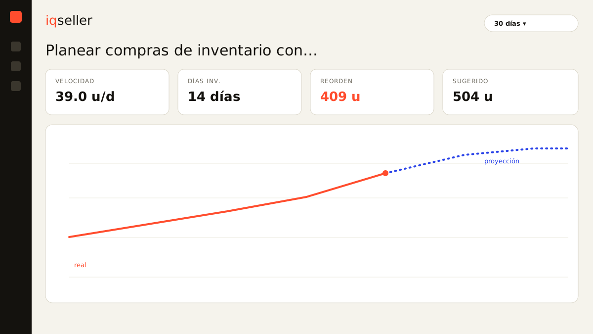
Forecast gives you sales velocity per SKU and per channel, the days of inventory you have left, the reorder point using the real lead time you’ve measured, and a replenishment recommendation over whatever horizon you define. That’s where the “how much” and the “when” of each product come from.

Profitability gives you real contribution per SKU: the COGS you loaded, commissions from the Amazon settlement and from MercadoLibre orders, FBA and Full fees, shipping, advertising, and the VAT and withholding breakdown. That’s where “how much each peso leaves” comes from.

Crossing the two is what turns a list of products in red into an order of priority. And the Inventory module closes the loop with real-time valuation: how much capital you already have placed, where it is — FBA, Full, 3PL, your own warehouse, in transit — and which part hasn’t moved in months. That last figure is usually the one that frees up the most budget, because the first source of capital for this month’s purchase is rarely a loan: it’s the dead inventory still taking up space in the warehouse and on your balance sheet.

On the Parent → Model → SKU tree, the ranking also stops looking like a flat list of codes and starts telling a story: which models carry the business, which variants within a model justify replenishment, and which ones should never have been listed.

one review per cycle, not one per year

The last point is about frequency. A purchasing plan under limited capital isn’t an annual document: it’s a decision retaken every time there’s money to buy.

Between one cycle and the next, everything feeding the ranking moves. Velocity shifts, fees change, a competitor drops a price and your contribution on that SKU shrinks, the supplier raises cost, lead time stretches. A ranking from three months ago is already describing a different business.

The discipline worth keeping is rebuilding the full list every time, even if it takes an hour, and comparing the new order against the previous one. SKUs that jump or drop several positions at once are almost always telling you something you hadn’t seen: a product that started turning, one whose margin got eaten, one whose lead time broke. That contrast between successive rankings is, in practice, the best early warning system an inventory business has.